home
needs
local resources
comfort
safety & health
contact
reports
Mathematical modeling of the total stove system
The discussion so far has concentrated on the individual aspects of heat transfer and fluid flow in a closed stove. We shall now turn to the problem of mathematical modeling of the complete system. The processes in a stove are essentially dependent on time and space variables. To take these into account in an exact manner is far too complex and the benefits one will get from solving an elaborate system of partial differential equations has to be doubted. This is particularly so if we note that most of these equations will require many constants whose values in a combustion system are at best known only approximately. What is more the geometries one encounters in a stove are not amenable to simple descriptions. Thus it is expedient to hold the mathematical development to relatively simple formulations.
The first simplification we will make is to replace the time dependence by time averages and treat the whole process as a steady state one. We further give up the idea of calculating flow and heat transfer as a function of space variables. Instead we divide the stove into a few well chosen sub regions in which the the flow and heat transfer variables are treated as constant. In chemical engineering practice this procedure is usually referred to as the well-stirred reactor model. In modern computer modeling work it is called the control volume approach. Except in the latter case a very large number of control volumes are used; we restrict ourselves to very few. For each of these sub-regions we draw appropriate force and energy balances. Thus the whole problem reduces to the solution of a set of algebraic equations. While these in principle could be carried out on a simple pocket calculator, availability of a PC with one of the more common spread-sheet programmes will come in handy to investigate a large number of variables concerning the design and operating characteristics.
In this section we shall present one example of analysis - for a single pan shielded fire. Kumar et al (1990) present a model for a multi-pan heavy stove.
The model of Delepeleire - Christiaens was modified by Bussmann and Krishna Prasad (1986) and Bussmann (1988) so that it becomes applicable to a shielded fire. In addition the model accounts for combustion temperature variations that occur due to variations in air flow through the stove caused by changes in flow resistances due to changes in gap widths between the shield and the pan. Figure 1 shows a schematic sketch of the stove with the nomenclature used in the analysis. The gas flow path is divided into four segments for purposes of modeling the flow and heat transfer.
- (i) The contraction and the bend from the flames (1) to the gap between the pan bottom and the combustion chamber top (2).
- (ii) The expansion in the gap under the pan from (2) to (3).
- (iii) The contraction/expansion at the pan bottom corner from (3) to (4).
- (iv) The annular gap between the pan side and the shield from the pan bottom (4) to the exit (5).
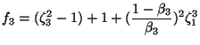
The first step in the model comprises of estimating the combustion temperatures using two overall energy balances. The first one is on the fuel bed and is the same as eq.(6.7) and we reproduce it below.
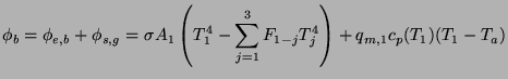 |
Due to the presence of radiation this is a nonlinear equation.
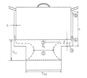
Fig.1. The Schematic Diagram of a Shielded Fire
In the calculations that follow ![]() is taken as the mass flow rate of
combustion gases corresponding to stoichiometric relations.
is taken as the mass flow rate of
combustion gases corresponding to stoichiometric relations. ![]() is
evaluated by taking 20% as the fixed carbon content of the wood and the
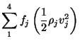
combustion value of carbon. The second heat balance evaluates the
temperature of the flames by invoking thermodynamic equilibrium .
is
evaluated by taking 20% as the fixed carbon content of the wood and the
combustion value of carbon. The second heat balance evaluates the
temperature of the flames by invoking thermodynamic equilibrium .
| (1) |
where
![]() ,
,
![]() stoichiometric mass of air for combustion.
stoichiometric mass of air for combustion.
The above equation was simplified by ignoring radiation losses from the
luminous flames and assuming complete combustion (ie,
![]() ). The equation then leads to an expression for
). The equation then leads to an expression for ![]() as a
function of
as a
function of ![]() .
.
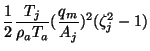
The second step in the procedure involves the calculation of flow resistance and draft. In the present model the density differences in each of the flow segments have been ignored. From the geometry shown in fig. 6.30 the following area ratios can be defined.
 |
(2) |
The general expression for the pressure change follows from Bernoulli's
equation
| (3) | |||
 |
(4) |
In practice extra pressure drops occur due to:
- (i)
- separation of flow downstream of bends and at the sharp edges of sudden contractions;
- (ii)
- Carnot losses at sudden expansions; and
- (iii)
- viscosity.
For the four segments the friction losses are determined according to the following formulae.
For the flow in segment (i) the friction factor is given by
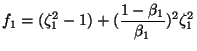 |
for |
(5) | |
| for |
(6) | ||
| (7) |
where
![]()
In segment (ii) the flow gradually expands from (2) to (3) as can be seen
from fig.6.29. Carnot losses occur for angles of expansion larger than ![]() radians. The friction factor for this case is given by
radians. The friction factor for this case is given by
| (8) |
The segment (iii) comprising of flow from region (3) to (4) is characterized
by a bend of ![]() radians followed by a contraction/expansion.The
pressure loss depends on the shape of the duct and is proportional to the
change in direction. The friction factor for this bend is taken as unity.
The friction factors for contraction / expansion is evaluated in a manner
similar to what was done in segment 1. This leads to the following
expressions for the friction factors in this segment:
radians followed by a contraction/expansion.The
pressure loss depends on the shape of the duct and is proportional to the
change in direction. The friction factor for this bend is taken as unity.
The friction factors for contraction / expansion is evaluated in a manner
similar to what was done in segment 1. This leads to the following
expressions for the friction factors in this segment:
 |
(9) | ||
| f |
(10) | ||
| (11) |
The friction factor in the annular region of segment (iv) is calculated assuming laminar flow. The annulus is approximated by a parallel plate geometry. This is permissible since the annulus width is much smaller than the radius of the pan. The second approximation involves the fact that the flow is developed. This is a more serious approximation in the sense that the pressure losses in a short duct will be larger than that for a very long duct.
| (12) |
where
![]()
This factor when multiplied by the dynamic head provides the pressure loss per unit length of the annular passage. To obtain a compact presentation we shall define the friction factor for the segment (iv)
| (13) |
where ![]() is the height of the annular passage (see Fig.6.29).
is the height of the annular passage (see Fig.6.29).
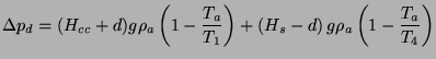
Thus the total pressure loss in the system is given by
 |
(14) | ||
 |
(15) | ||
| (16) |
where
![]() and
and
![]()
This pressure loss and the dynamic head corresponding to the escaping velocity of the gases from the stove have to be balanced by the draft which is calculated according to
 |
(17) |
Thus
| (18) |
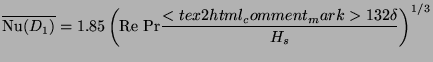
We now turn to the heat transfer calculation. There are two parts to this calculation: (i) pan bottom; and (ii) pan side. The pan bottom heat transfer is calculated according to the stagnation point heat transfer correlations given by
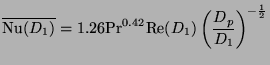 |
(19) |
![]() is the pan diameter and
is the pan diameter and ![]() is the diameter of the plume at
section (1) in Fig.6.30 and is estimated on the basis of the open fire model
described in the flame heights page. The other symbols have been defined
earlier.
is the diameter of the plume at
section (1) in Fig.6.30 and is estimated on the basis of the open fire model
described in the flame heights page. The other symbols have been defined
earlier.
For the pan side the arguments are more involved. There are three separate approximations involved. Firstly the geometry is approximated by the parallel plate configuration (same as we used for the friction factor calculation). Secondly neither the flow nor the heat transfer can be considered as fully developed. As we shall discuss later it is sufficient for the purpose of stove work to treat the problem as one of hydrodynamically developed flow and thermally developing system. Finally the temperatures of the pan and shield will not only be different but will vary along the height. Since the purpose here is to demonstrate the relative importance of the heat transfer coefficient and the excess air factor in determining the heat absorption by the pan, we consider the simplest case of holding the shield temperature to be uniform and equal to that of pan. We shall towards the end of this section relax a few of these assumptions and present some results obtained from the more complex model. For the approximations listed above one can use the following correlation proposed by Shah and London (1978).
 |
(20) |
Once the Nusselt numbers are known the heat transfer can be found from
| (21) |
![]() is the logarithmic mean temperature difference defined by
is the logarithmic mean temperature difference defined by
 |
(22) |
![]() and
and
![]() are the temperature differences at inlet
and exit to the shield region of the stove. In the various equations above
the properties are evaluated at the corresponding average temperatures.
are the temperature differences at inlet
and exit to the shield region of the stove. In the various equations above
the properties are evaluated at the corresponding average temperatures.
The set of equations (6.7) and (6.26) through (6.42) are used to evaluate
- (i)
- the excess air factor,
 ;
; - (ii)
- the temperatures
 ,
,  and
and  ; and
; and - (iii)
- the heat transfers
 and
and  .
.
The parameters investigated are:
- (i)
- the pan-shield gap;
- (ii)
- the combustion chamber top-pan bottom gap;
- (iii)
- the shield height;
- (iv)
- the pan size; and
- (v)
- the power output of the fire.
The following parameters were held constant: ![]() = 180 mm; and
= 180 mm; and ![]() = 100 mm
= 100 mm
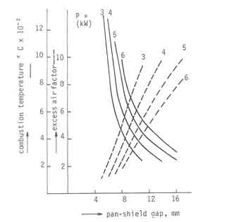
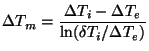
Fig.2. Calculated excess air factors and combustion temperatures
Figure shows the combustion temperatures and excess air factors as a
function of pan-shield gap and power output of the fire for a pan of
diameter 280 mm and a shield height of 150 mm. The power range investigated
corresponds to grate power density in the range 12 to 24
![]() . Solutions outside the range 1 <
. Solutions outside the range 1 < ![]() < 10
were rejected as physically unrealistic. Four results emerge from a study of
this figure. Firstly, at a given power level, increase in gap width results
in enormous increases in excess air. Correspondingly one notices steep
reductions in combustion temperature. Secondly, as the power level
increases, the minimum gap necessary to avoid the fire being starved of air
increases. This result brings out an important feature of wood burning
devices. Consider a stove designed to operate at 6 kW. It requires a minimum
pan-shield gap of 8 mm. If such a stove is operated at 3 kW the excess air
factor increases from about 1.75 to about 5 with the combustion temperature
going down from 975 C to 450
< 10
were rejected as physically unrealistic. Four results emerge from a study of
this figure. Firstly, at a given power level, increase in gap width results
in enormous increases in excess air. Correspondingly one notices steep
reductions in combustion temperature. Secondly, as the power level
increases, the minimum gap necessary to avoid the fire being starved of air
increases. This result brings out an important feature of wood burning
devices. Consider a stove designed to operate at 6 kW. It requires a minimum
pan-shield gap of 8 mm. If such a stove is operated at 3 kW the excess air
factor increases from about 1.75 to about 5 with the combustion temperature
going down from 975 C to 450 ![]() C. Drastic reduction in
efficiencies can result. Needless to say there is a control aspect as well
here which we shall elaborate in the page on controls. There is a more
important aspect here. If it is desired to operate the stove in the range of
power outputs from 3 to 6 kW, the permissible range of gap widths is only
between 8 and 11 mm. This is an extremely severe restriction on the design
if we note that the manufacturing tolerances of this level are currently
unavailable for stove producers.
C. Drastic reduction in
efficiencies can result. Needless to say there is a control aspect as well
here which we shall elaborate in the page on controls. There is a more
important aspect here. If it is desired to operate the stove in the range of
power outputs from 3 to 6 kW, the permissible range of gap widths is only
between 8 and 11 mm. This is an extremely severe restriction on the design
if we note that the manufacturing tolerances of this level are currently
unavailable for stove producers.
Figure 3 shows the results of the heat transfer coefficient calculations for the pan bottom and the pan side for the same set of parameter values as in Fig.1.
Fig.3. Calculated heat transfer coefficients
A striking feature of the plot is that the heat transfer coefficients for
the whole range of parameters lie in a narrow range of12.5 to 20 W/m![]() C. The variation for the pan side is somewhat larger than that for the pan
bottom. This is as it should be since the parameters investigated have been
chosen to concentrate the flow resistance in the pan-shield gap. Further the
pan bottom heat transfer coefficient shows a pronounced maximum. The reason
for this requires further investigation. The most important conclusion to
emerge from these results is that a four fold increase in the pan-shield gap
reduces the heat transfer coefficient by about a third. This is in strong
contrast to the gap effect on excess air and combustion temperatures which
is much stronger.
C. The variation for the pan side is somewhat larger than that for the pan
bottom. This is as it should be since the parameters investigated have been
chosen to concentrate the flow resistance in the pan-shield gap. Further the
pan bottom heat transfer coefficient shows a pronounced maximum. The reason
for this requires further investigation. The most important conclusion to
emerge from these results is that a four fold increase in the pan-shield gap
reduces the heat transfer coefficient by about a third. This is in strong
contrast to the gap effect on excess air and combustion temperatures which
is much stronger.
In order to get a total picture we need to look at the heat transfer results which we shall now turn to. The heat transfer to the pan comprises of three distinct parts.
- (i)
- Radiative heat transfer to the pan bottom.
- (ii)
- Convective heat transfer to the pan bottom.
- (iii)
- Convective heat transfer to the pan side.
In these calculations it has been assumed that the ratio between the radiative heat transfer to the pan bottom and the heat liberated by combustion is constant and independent of the power of the fire. As per measurements of Herwijn (1984; ) on open fires this constant is 0.13. No similar measurements are available for the shielded fire and we have to satisfy ourselves with the open fire result. With this assumption one can easily compute the heat transfer and the results are plotted in Fig.4 as efficiencies again for the same set of parameters as in the previous two figures.
Fig.4. Calculated efficiencies compared with measured efficiencies as a function of pan-shield gap
The expected decreases in efficiency with increasing gap width are
reproduced by the calculations.
Three other features emerge from this plot. The efficiency in the operating
range of gap widths is not a strong function of power output of the fire.
This has been earlier demonstrated for the open fire (see Fig.. ). This has
also been measured for a wide variety of stoves as can be seen from Fig.5
which was assembled by Sangen (1983). A superficial observation suggests
that the efficiency drops with increased gap widths calculated according to
the present model are nowhere near the ones suggested by the
Delepeleire-Christiaens model (see Fig.6.26). However it must be pointed out
that the results in Fig.6.26 are not easy to interpret in terms of the
parameters considered in the work of Bussmann and Krishna Prasad. Since the
heat flux density is not an easily measurable quantity, it is preferable to
use the method indicated in Fig.6.33. The third feature concerns the
convective heat transfer to the pan bottom which is also plotted in Fig.6.33
for a 4 kW fire. It is seen that the efficiency decreases as the shield-pan
gap width increases. Since the pan bottom and the combustion chamber top gap
was held constant in these calculations the reduction in heat transfer has
to be attributed to the increased pan-shield gap widths resulting in
increased air supply with consequent reduction in combustion temperature.
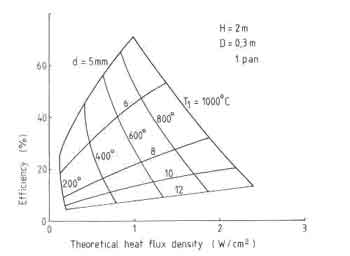
Fig.5. Stove efficiencies according to Delepeleire - Christiaens model Efficiencies of Several Stove Designs
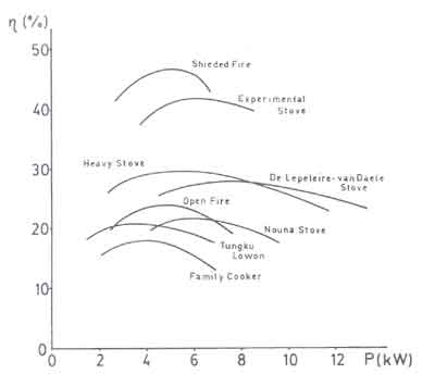
Fig.6. Efficiencies of Several Stove Designs
A fairly comprehensive programme of measurements carried out by van Dijk (1985) and van der Donk (1985) are available for comparison with the above theoretical results. These are also shown in Fig.6.33. The detailed dimensions of the stove used in these experiments are shown in Fig.7. The most important characteristic of these stoves is that they had fairly large air admission holes so that the resistance to air flow through the stove was concentrated in the important heat transfer regions.
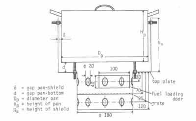
Fig.7. Dimensions of the stove used by van Dijk and van der Donk
These experiments use oven dry white fir cut in pieces with size 20x20x67
![]() . The efficiency measurements at a power output of 4 kW are
included in Fig.6.33. It is interesting to note that the theory in spite of
the very gross assumptions made in its development - the most important of
which are the treatment of combustion as a steady state process and a
spatially invariant temperature of the combustion products - compares
reasonably well with the experiments. The maximum deviation between the
theory and experiment is about 26% in a relative sense.
. The efficiency measurements at a power output of 4 kW are
included in Fig.6.33. It is interesting to note that the theory in spite of
the very gross assumptions made in its development - the most important of
which are the treatment of combustion as a steady state process and a
spatially invariant temperature of the combustion products - compares
reasonably well with the experiments. The maximum deviation between the
theory and experiment is about 26% in a relative sense.
A second type of experimental arrangement was constructed to explicitly determine the amount of heat transferred to the pan bottom and pan sides (Fig.8). The results of these are also plotted in Fig.4. The relative deviation of the theory from the experiment are substantially larger. The theory suffers on two counts.
- (i)
- The experiments do not show the rapid decrease in efficiency with increasing gap widths. This is probably caused by the improper estimation of resistances and draught in the theory.
- (ii)
- In the pan side heat transfer the theory shows a rather sharp cutoff point at the low gap widths and this is absent in the experiments. This is hard to explain on the basis of the presently available information.
A final comment about the comparison between the theory and experiment concerns the experimental arrangement used to infer the pan side heat transfer.
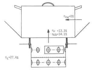
Fig.8. Experimental Arrangement for the determination of heat transfer to the pan bottom
The fact that the pan bottom heat transfer drastically reduces with the reduction of the shield-pan gap invalidates this arrangement.
The major conclusion to emerge from this study is that geometrical changes in the stove design has very pronounced influence on the flow through the system. This influences the combustion temperature considerably which in turn has a decisive role in determining the efficiency of the stove