EXPERIMENTAL TECHNIQUES

Introduction

The combustion of wood is a complex phenomenon. As a result studies on wood combustion are still almost entirely empirical. Emmons (1983) states that:

''The current scientific understanding of the combustion of wood is not mature enough to provide quantitative prediction, but, nevertheless, is very useful for providing direction. The final design of a stove -should be determined experimentally for the available bio-fuel guided by what is currently known of the science of fire''.

Emmons, thus, emphasizes the need for experimental work in designing stoves.

First the test methodology will be presented, which is used in the WSG laboratory experiments. The presentation is followed with a discussion on the relevant quantities

The WSG test Procedure

The WSG test procedure for woodburning cookstoves presented in this section is based on the methodology for testing gas ranges (GIVEG 1968). Using a procedure similar to the GIVEG methodology means that:

• (i)         the maximum power of the stove must be determined;
• (ii)        the turn down ratio, the ratio between maximum and minimum power must be measured;
• (iii) water boiling tests have to be performed, in order to measure the efficiency of the stove as a function of the power; and
• (iv)        it must be determined whether or not the stove meets the safety

requirements.

The main difference compared with testing gas ranges, is that wood is a solid fuel of non-uniform quality which is not available on tap. The fuel quality is used as a catch-all term to denote the wood species, the as-fired moisture content of the wood, the size of the wood actually employed in the fire etc. The results of a series of experiments will not match when fuel parameters are varied in addition to the variable actually examined. The consequence is that experiments have to be subjected to a well defined scheme of fuel preparation and fuel loading. When this scheme is followed, it will lead to experimental results which are highly reproducible.

The experimental procedure unless otherwise specified is as follows. White fir wood is cut into pieces of 20*20*67 mm ³ and dried to constant mass in an oven at 105 ° C (±48 hr). The wood is then divided into lots of 100 grams each, which are charged to the fire at fixed time intervals. The fire is built on a grate with a diameter of 0.18 m. At the start of the experiments the fire is lit with a propane burner (±30 s). The experiments stop when all the wood has been burnt. In the experiments 5 kg of water in a pan 0.13 m above the fuelbed is brought to the boil and is kept boiling. Some water will evaporate and escapes as steam. The pan is made from aluminium, has a diameter of 0.28 m, a height of 0.24 m and is always used with a lid.

The power output

Nominal and average power

It is common practice to test heating devices at constant power (burning rate). In the present case this demands a steadily burning fire. One way of obtaining such a fire is by adding small quantities of wood at short time interval, but this is a cumbersome procedure. However the stove can be considered to burn in a steady periodic way when bigger charges ( ) are added at larger time intervals ( ). For such a batch process, a nominal power can be defined according to the formula:

In general the nominal power of a fire of a given configuration can be varied within certain well-defined limits by changing or both.

A problem arises due to the build-up of charcoal in the fuelbed. This results in the water continuing to boil even after the last wood charge has been burned away. Since the end of the water boiling test is defined as the moment of time the water stops boiling ( ), it raises the question whether it is not better to use a power definition based on this time, 'leading to the concept of an average power.

The data presented in the table are from experiments performed on the open fire. The extent of the difference between nominal and average power can be taken as a measure of the charcoal heat available with a given stove configuration. It is a function of power, fuel type, moisture content and wood block size. In general the difference between nominal and average power increases as the power of the fire increases. The influence of the moisture content and the wood species is erratic; too few experiments were performed to draw any firm conclusions.

Adding the wood in charges creates another unexpected problem. Changing the mass of wood charged or the charge time interval. in order to vary the power. has completely different effects on the fire behaviour. This is illustrated in the Fig.1, where the carbon dioxide content in the flue gases is given as a function of time, 1a, where the charge weight is varied and the peak values of the carbon dioxide concentration curve change accordingly, and lb where. on the other hand, the charge time is varied but the peak values in the carbon dioxide concentration increase until. during the last charge of the three experiments, they all attain about the same level.

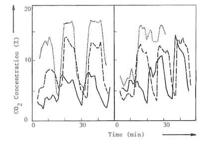
a: Charge weight varied	... 9.0 kW	- - - 6.3 kW	--- 3.4 kW
d: Charge time varied	... 9.5 kW	- - - 6.0 kW	--- 4.0 kW

Fig.1. Carbon dioxide concentration versus time for three nominal powers

The time dependent power output

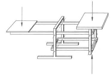
The phenomena shown in Fig.1 cannot be explained on the basis of the average and/or nominal power. There is clearly a need to obtain a better understanding of the time dependent burning process. To that end the experiments are performed on a platform balance in order to record the weight of the fuelbed as a function of time. The balance is shown in figure 2; it was designed in such a way that, first, the recorded signal was insensitive to the position of the fire on the platform; and, second, the mass of the stoves (upto 60 kg) could be balanced completely by counterweights. The equipment was insensitive to temperature changes and had an accuracy of one gram (Visser 1982).

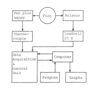
Every ten seconds the weight of the fuel was measured. This measuring and gathering of data was done by means of a data acquisition unit (HP 3497A) controlled by a microprocessor (HP 85). After measuring, the data were stored on tape which was processed after the experiments. The set-up of the measuring system is shown schematically in Fig.3.

The record of the fuelbed weight is a valuable tool for understanding wood fires in operation. In general, after an initial period of unsteady operation, 'a periodic steady state' regime of burning will be established. In this regime the weight loss curves will be congruent with one another - of course this will not be achieved in a strict mathematical sense.

A characteristic picture of the fuelbed behaviour of the open fire subjected to the charging procedure is given in Fig. 4a. The figure shows the fuel weight as a function of time. The experimental procedure is as follows. At time t=t a charge is added to the fuelbed. This charge catches fire and burns until. at time t=t . A fresh charge is added, and so on. The refuelling, at t=t , does not always mean that the wood charged at t=t has burned completely. Figure 4a shows, for instance, that the amount of wood left from the third charge is equal to gram. In the graph the accumulated mass of unburned wood just before recharging becomes larger as time progresses and is equal to gram at the end of the experiment. This process is called the fuelbed build-up.

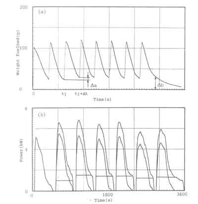
The weight-loss records can be utilized for estimating the actual time-dependent power output of the fire. The primary assumptions behind these estimates are that the combustion of wood takes place in two phases (solid phase combustion of charcoal and gaseous phase combustion of volatiles) and that the fuelbed only consists of charcoal and ash. This latter assumption is valid for the entire combustion process at low nominal powers and for the steady state period at modest nominal power levels. For large nominal power levels however this is not true; the fuelbed will consist of wood in various stages of thermal decomposition. It would be pure speculation to attempt to identify the proportion of charcoal and volatiles burnt for each charge with the present experimental technique. However, it is quite inefficient to operate a stove of a given configuration at such high nominal power levels. A final assumption concerns the charcoal combustion rate which is taken to be constant during the period between two fuel loadings. In reality this may not be the case. However. since the calculated point of time at which the power of volatiles becomes zero synchronizes with the disappearance of the flames, the assumption mentioned is good as a first approximation (see Appendix 1 for a more elaborate discussion).

On the basis of the assumptions made, the time-dependent powers P(t). P (t) and P (t) can he obtained by multiplying the separated mass flows with their proper combustion values. A sample result of refashioning the fuelbed weight data In the way described above has been given in figure 4b. The figure shows the rate of heat output of the fire subdivided into the contributions from the charcoal as well as from the volatiles. The lowest, block-shaped, curve represents the rate of heat output of the charcoal, P (t). The lower of the parabola shaped curve represents the rate of heat output of the volatiles, P (t) while the topmost curve shows the total rate of heat output. P(t). The charcoal heat output being block-shaped is a result of the assumed constant charcoal burning rate.

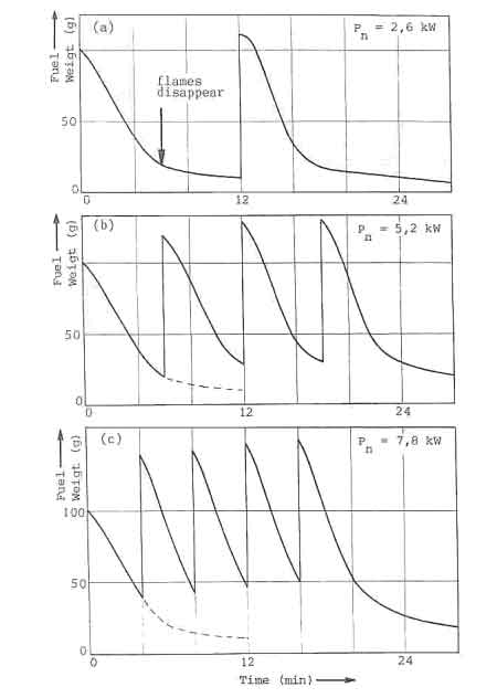
The maximum power

The discussion so far showed the problems in defining the power output. On top of this, criteria have to be found which make it possible to rate the power of a stove. The criterion used so far is the excessive build-up of the fuelbed. The nature of this is shown in figure 5 where the fuelbed weight of the open fire on a grate is given as function of time for three different nominal power levels. In the experiments the variations in power have been accomplished by changing and holding constant. On the basis of a change in slope it is possible to distinguish two regions in the weight-loss curve of each charge. The point at which a drastic change in slope occurs in general coincides with the disappearance of flames (the point is marked in figure 5a). After this point only the charcoal in wood burns. Figure 5c then shows that a fresh charge is added even before the flames disappear when the nominal power is raised to 7.8 kW. It leads to a rapid build-up of the fuelbed. Attempts to increase the power beyond that of 7.8 kW result in the fuel falling off the grate. The corresponding situation for an open fire without a grate - driving a fire above a maximum power limit - will result in an increased fuelbed diameter. For a closed stove, exceeding the high power limit results in the choking of the combustion chamber with fuel. A given design of a stove will thus permit a well defined range of power to be obtained from it.

(a) P 2.6 kW; (b) P 5.2 kW; (c) P 7.8 kW

Only recently the criterion of the excessively high carbon monoxide to carbon dioxide ratio came into the picture. Many more experiments to collect data in this field are needed.

The minimum power

Criteria also have to be evolved which determine the minimum power or the turn down factor. The task to perform at minimum power levels is to balance the convective, radiative and evaporative heat losses from the pan in the simmering period.

The convective heat losses are given by:

The size of the pan area losing convective heat (A ), depends on the position of the pan on/in the stove. The heat transfer coefficient for the pan wall and lid (h ) can he calculated using the Nusselt number relations for free convection (Kreith & Black 1980):.

where:        C = 0.15 and n = 1/3 for the lid; and

                 C = 0.59 and n = 1/4 for the pan wall

When the cooking is done in a windy environment, the above Nusselt number relations must be replaced by those for forced convection.

The radiative losses are given by:

The losses depend on the emissivity of the pan surface which can vary from nearly 0, for bright shining aluminium surfaces, to 1 for black surfaces (Eckert & Drake 1972).

Finally, the evaporative heat losses are given by:

The evaporation rate (m ) depends on the difference between the saturation pressure at boiling and ambient temperature. Using modified forms of the Clausius Clapeyron equation (Irvine and Liley 1984), the rate is given by:

kg/s         (7)

where C C and p

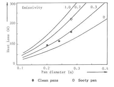
A series of experiments was performed to determine the convective and radiative heat losses from standard pans with a lid (GIVEG 1968). Water in the pan was heated with an immersion heater: and the temperature rise was recorded as a fuction of time and power of the heater. The measured heat losses from three different sized pans at 97C are shown in Fig.6 as solid dots. The experimental data In the figure are compared with calculated curves. In the calculations it is assumed that evaporation can be neglected due to the use of lids. The average emissivity of the pan surface has been varied parametrically (0, 0.3, 0.7 and 1 respectively). Good agreement between theory and experiment is obtained for an emissivity of 0.3. This value is judged reasonable for the corroded aluminium Pans used in the experiments, one experiment. also shown in the figure, has been repeated with a sooted pan. The radiative losses increased considerably; an average emissivity of 0.7 is then needed in order to obtain agreement with the calculations

The calculated heat losses from standard pans with a lid, having an emissivity of 0.3, receiving heat from the bottom only, placed in wind-free surroundings. and at boiling temperature, are shown in Table 2.

The heat losses shown in the table, divided by the efficiency of the stove, give the minimum powers required to keep the food simmering. In the last column of the table this was done for the improved stoves disseminated in Niger which have an efficiency of ± 30%. On the basis of Table 2, and knowing the maximum power of the stoves in Niger (ranging from 4 kW to 12 kW) it is concluded that the stoves should have a turn-down factor of 10. In reality the turn-down factor ranges from 3 to 4 and consequently the design has to be improved on this part. The designer should aim at a minimum turn-down factor of at least 6; a value specified in the GIVEG standard for gas ranges.

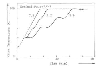
The required minimum power level for open fires and improved stoves without air control, can not be obtained by simply decreasing the charge size and increasing the charge time. In Fig.7, this is illustrated for the open fire. The figure shows the water temperature response in the experiments discussed before (Fig. 5). At a nominal power of 2.6 kW, the temperature curve exhibits distinct plateaus that correspond roughly to the disappearance of flames. The power level obtained from the charcoal bed apparently is sufficient to balance the heat losses from the pan. Thus for simmering conditions the power should be reduced to this level. However, in the experiments any attempt to lower the nominal power below 2.6 kW resulted in an insufficient quantity of burning charcoal on the fuelbed for a fresh charge to reignite without the assistance of an external pilot flame.

The foregoing suggests that improved stoves should be able to separate the volatiles and charcoal combustion. the charcoal being used during the simmering period. In all the (one hour) experiments with the open fire reported here. the water kept boiling after the flames disappeared for a little over 6 minutes at the low power end and 17 minutes at the high power. However, In some of the experimental closed stoves tested by the Eindhoven/Apeldoorn group, this charcoal heat is sufficient to keep the water boiling for over 30 minutes (Nievergeld et al, 1981; Vermeer & Sieleken 1983). In this way, the charcoal heat can contribute to substantial savings in the fuel consumption.

The heat losses during simmering become much larger when lids are not used and evaporation cannot he neglected. A series of experiments was performed to determine the heat losses from 280 mm diameter pans under similar conditions as the experiments with lids discussed before. A constant heat flow was supplied to the water with an immersion heater and the resulting steady state temperature was measured. The experimental data are presented in Table 3

The steady state temperature was used to determine the constant C, of the evaporation rate equation 7, where after the evaporative heat losses at boiling point were then calculated. The table below shows the results for three different power levels of the immersion heater.

The results of table 3 are consistent. The calculated heat losses only vary by less than 5%. This justifies the modelling of the evaporative losses as discussed. Comparison of the tables 2 and 3 shows that the heat losses at boiling point can be reduced by a factor of six when evaporation is prevented, i.e when lids are used and the power is adjusted.

The design power

The power of the fire peaks after fresh wood is added. A stove must get through this power peak with a reasonable combustion quality. A sufficient amount of combustion air must be supplied. In designing stoves this has led to the definition of the design power (P ) which is the maximum nominal power that a stove can deliver under steady state operation. Experiments on open fires showed that the design power is about 70% of the peak power mentioned above . It is feasible to operate open fires with a nominal power higher than the design power for durations of the order of 1/2 to 1 hour. It can be expected that closed stoves exhibit similar tendencies In their operation (see for example Delsing (1981) for non-chimney closed stove operation qualitatively illustrating fuelbed build-up). However, when closed stoves are operated at powers exceeding the design power on a regular basis, they will demand frequent maintenance by way of the removal of tarry deposits in passages and from the internal walls of the stove. When this maintenance is not provided, the performance may deteriorate rapidly and may even lead to drastic reductions n the lifetime of stoves. Thus for safe and durable operation of a stove, it is essential to operate it at, or near, its design power level.

Formula 8 finally shows how P can be thought of as being built-up from the charcoal and volatiles powers, P and P respectively.

Earlier it was argued that P is constant during a charge interval. For steady state operations, and assuming a fixed carbon content In wood of 20%, this implies that:

P = 0.32 P

P on the other hand is the average value of the volatile powerpeaks recorded In the weight loss experiments. P will play an important role in analysing the experimental data on open fires.

The efficiency

The efficiency is a measure of the heat transferred from the stove/fire to the pan(s) under a regime of well-defined operational procedures. The efficiency is determined by a water boiling test as discussed earlier. The efficiency is taken to be the ratio between the heat absorbed by the water in the pan and the heat released by the wood under the assumption of complete combustion. The efficiency Is calculated using the formula:

Evaporation is not considered to be a loss, which has led to some confusion. In the standards of performance for domestic gas ranges the relevant experiments only last until boiling point is reached (CIVEG 1968). For wood stoves this would result in large experimental errors due to the fact that the fuel is not available on tap but must be charged in batches. Replacing pans once boiling point is reached might overcome this problem (Micuta 1982). However, as long as the work is restricted to measuring comparative efficiencies, what method is used to calculate those efficiencies is a trivial matter (Krishna Prasad 1981).

The efficiency depends on the pan size used. If the choice of pan and cooking task Is not restricted by the stove design, they are chosen according to the power rating; thus Fmax needs to be determined first. The rule of thumb for gas ranges is to have a heat flux through the pan bottom of 3.5 W/cm². At an efficiency of 50% this requires a power density at the pan bottom of 7 W/cm². For wood stoves the power density should be much higher as the efficiency is lover. Thus the x-axis in figure 2.8 has three different scales, representing power densities of 7 W/cm², 10 W/cm2 and 17.5 W/cm2 bottom area at efficiencies of 50%, 35% and 20% respectively.

2.5. The CO-CO2 ratio

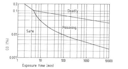
One of the major problems in designing improved stoves concern the combustion quality. In testing woodburning cookstoves this problem has almost been neglected entirely although Smith (1986) clearly showed the seriousness of the problem. The products of incomplete combustion are carbon monoxide, hydrocarbons and soot. Carbon monoxide especially deserves full attention when considering the stove performance. Sulilatu (1935) showed the poisonousness of this colourless and odourless gas. The effect of the carbon monoxide concentration in the atmosphere as a function of the exposure time for various conditions of labour are shown in Fig. 9.

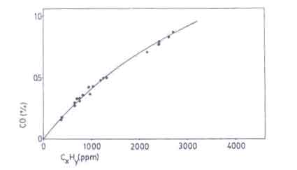
Sangen (1983) showed that the carbon monoxide content in the flue gases also correspond to the release of unburnt hydrocarbons (see Fig.10). This is also implicit in the more recent work of Dilip R.Ahuja et al. (1987). Since it is much more cumbersome to measure CxHy and soot, the carbon monoxide content has been taken as a quantity indicative of the combustion quality. In spite of this simplification, the experimental task of measuring the quantity of carbon monoxide emitted in non-chimney stoves is hard.

Fig.10. Relationship between carbon monoxide and C H concentrations

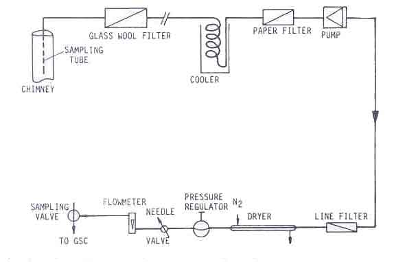
Absolute measurements of the carbon monoxide concentration in flue gases are only possible in closed stoves with a chimney. This is why for all practical purposes, the carbon monoxide to carbon dioxide ratio is used as an indicator of the toxicity of the combustion gases. It involves the measurement of both the carbon monoxide and carbon dioxide content. The experimental set-up is shown in Figure 11. (Sielcken 1983).

The methodology for testing gas ranges gives clear standards for the relative carbon monoxide content in the flue gases. In Table 4 the norms applied in the Netherlands for different burners are given. It is essential that the power is specified as well.

In Fig.12 the carbon monoxide to carbon dioxide ratio is shown as a function of the power for throe similar chimney stoves, with combustion chambers of different size. The carbon monoxide to carbon dioxide ratios were averaged over the water boiling experiment. In the figure the standards from Table 4 are shown too. Although the stoves show higher efficiencies than many other designs, their index of toxicity is dangerously high for the whole power range investigated. It shows the necessity for including the carbon monoxide and carbon dioxide measurements In the test methodology.

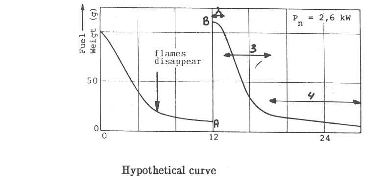
Fig.12. Carbon monoxide to carbondioxide ratio as a function of the nominal power.
Data from stoves with combustion chambers of different diameters

Appendix 1

The heat release rate of the fire

This appendix will discuss the method of computing the heat release rate from a steadily burning fire by using the wood weight-loss curves. The discussion centres around three possible assumptions on the rate of burning of charcoal in the fuelbed.

Figure A1 is a schematic representation of the weight-loss of a charge of i~Mf gram (Curve A). The slope of the curve is a measure for the burning rate of wood at each point of time. At the ez~d of the charging interval ItzAt). the fuelbed weight is 'a' gram. Under steady state operation. 'a' has the same value after each charge interval.

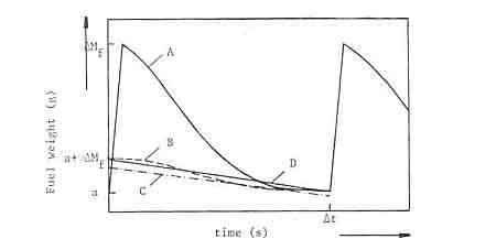
Fig A1: Schematic fuel weight-loss cui-ve of a wood fire

Three assumtopns about the burning rate of charcoal were considered:

1. The charcoal weight-loss curve is similar to the measured wood weight-loss curve (curve B in figure A1).
2. The charcoal burns at a constant rate during the whole period that flames are visible. This burning rate can be measured as soon as the flames disappear. In figure A1 the charcoal weight loss rate is represented by the straight line C.
3. The charcoal burns at a constant rate during the whole charge period. The rate is determined by the quantity of fixed charbori added in every charge (D.AMf) and the charge tune At. In figure Al this case is represented by a straight line between the known poinLs (0. a-I-v.kM~) arid (At, a). (line D in figure A1).

The first assumption has been rejected as unrealistic, According to Wagner (1978) there will be a phase difference between the burning cycles of charcoal and volatiles. A reasonable interpretation of the Wagner model is; that charcoal from the previous charge is used to drive the volatiles from the present charge of wood. The difficulty with the second assumption is that the point at wltich flames disappear cannot be unambiguously identified. Moreover the assumption results in calculated quantities of fixed charbon which differ somewhat from the results of the proximate analysis of the wood. The third assumption was therefore used in the calculations. It was found from an examination of many weight-loss curves that the line D after P (see figure A1) follows very nearly the total weight-loss curve.

A final comment needs to be made on the linearity assurnptiion. Experiments conducted with charcoal in a shielded charcoal burner showed weight-loss curves lhat are remarkably linear from the beginning to the end of the experiment as was shown in figure A2. This is an additional support for the assumption used in the analysis adopted in this investigation.

Back